Thanh Tu, Do

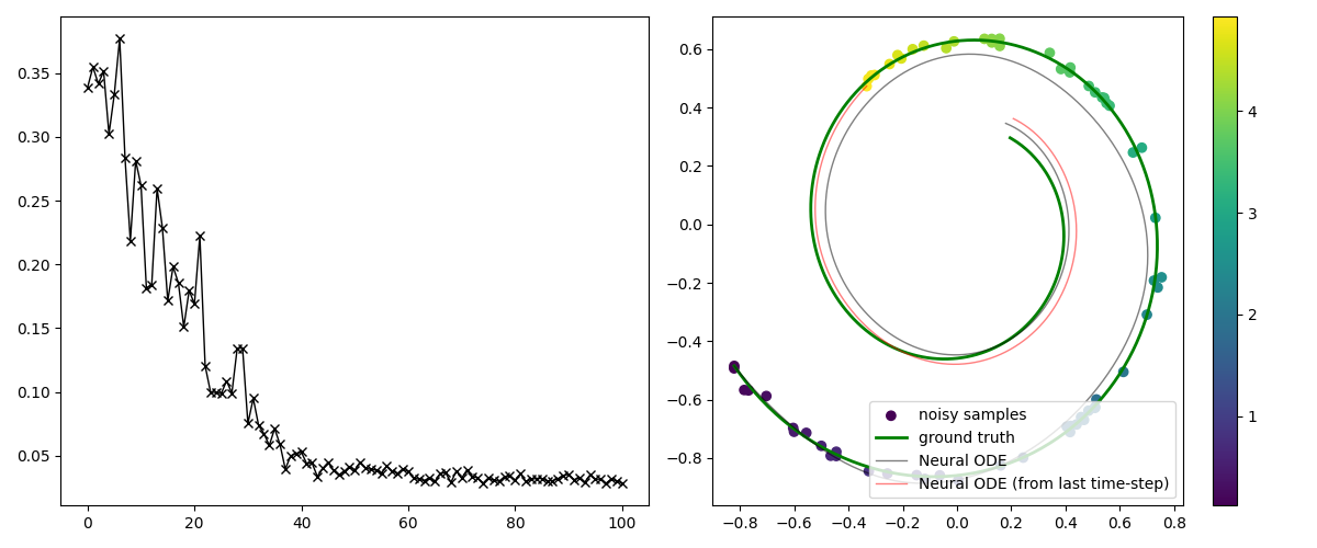
Motivation This blog post is my note taken when studying Neural Oridinary Differential Equation (NeuralODE), which was proposed in Neural Ordinary Differential Equations. The goal of this note is to understand the formulation, some mathematical derivations, and some techincal difficulties encounter when implementing NeuralODE in JAX. The entire learning process is quite fascinating and introduced me to some new mathematical concepts such as Euler-Lagrange equation, Continuous Lagrangian Multiplier. NeuralODE is a important entry point to Physics Informed Machine Learning and I struggled for quite sometime to understand....

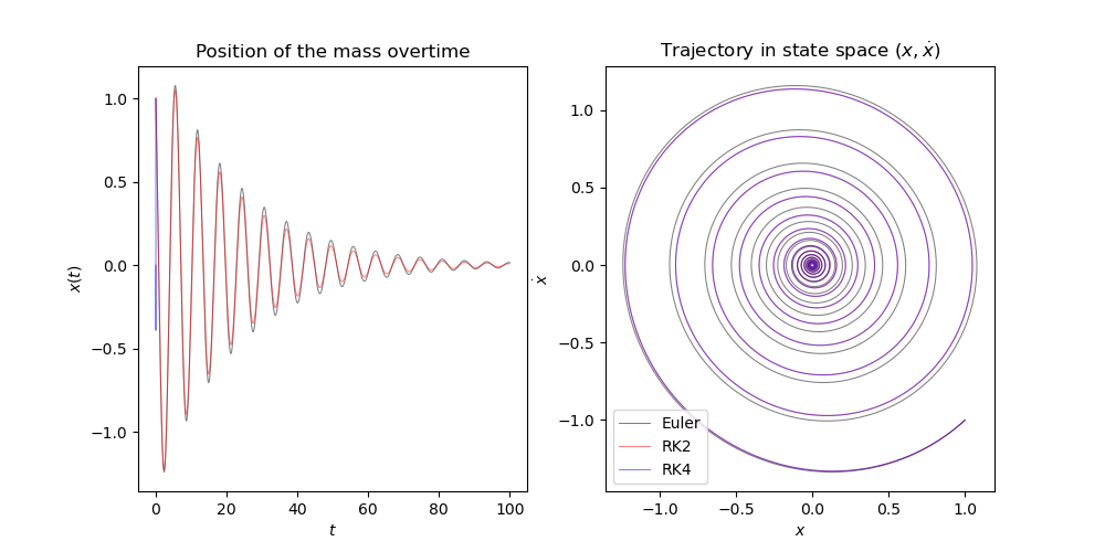
todo Derivation of second and forth order Runge-Kutta methods Comparison of truncation error with different step-size Ordinary Differential Equation (ODE) Initial Value Problem A differential equation is differential equation is a relationship between function \(f(x)\), its independent variable \(x\), and any number of its derivative. An ODE is a differential equation where the independent variable and its derivatives are in one dimension. $$ \begin{equation} F(x, f(x), f^{(1)}(x), f^{(2)}, \cdots f^{(n-1)}(x)) = f^{(n)}(x) \end{equation} $$...

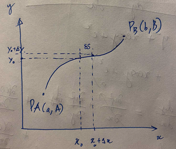
My goal for this post is to have a basic understanding of Calculus of Variations, so that I can be more comfortable with mathematics in NeuralODE paper, where the problem can be formulated as a optimization of a functional with ODE constraint (Adjoint State Method for an ODE). My first encounter with Calculus of Variation is one of my homework where we try to derive probablity density function of some distribution by the principle of maximum entropy....

Surveying numerical methods (finite difference methods) and physics-informed neural networks to solve a 1D heat equation. This post was heavily inspired by: (Book) Partial Differential Equations for Scientists and Engineers - Standley J. Farlow for deriving closed-form solution. (Article) Finite-Difference Approximations to the Heat Equation (Course) ETH Zurich | Deep Learning for Scientific Computing 2023 for Theory and Implementation of Physics-Informed Neural Network. Introduction Physics-Informed Machine Learning (PIML) is an exciting subfield of Machine Learning that aims to incorporate physical laws and/or constraints into statistical machine learning....

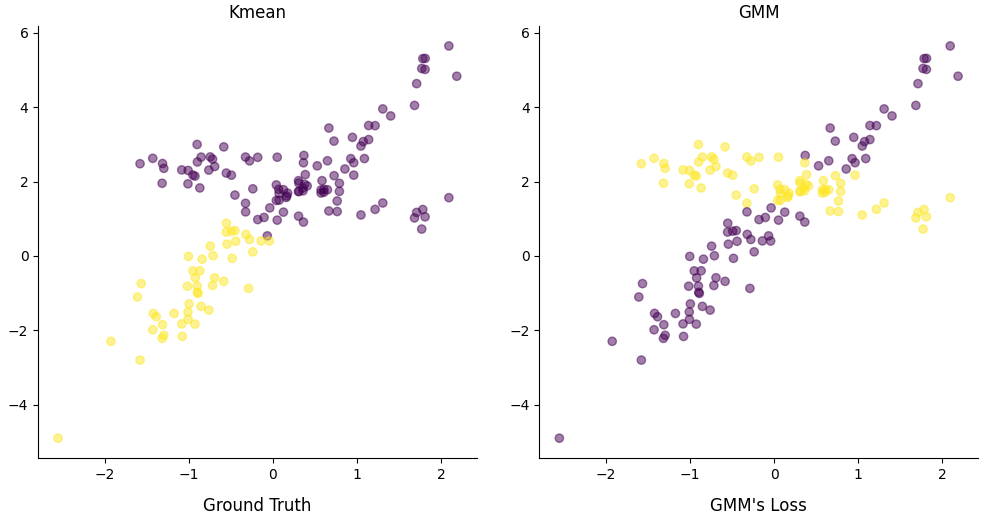
Problem Given a statistical model \(P(\boldsymbol{X}, \boldsymbol{Z} | \boldsymbol{\theta})\), which generate set of observations \(\boldsymbol{X}\), where \(\boldsymbol{Z}\) is a latent variable and unknow parameter vector \(\boldsymbol{\theta}\). The goal is to find \(\boldsymbol{\theta}\) that maximize the marginal likelihood: $$ \mathcal{L}(\boldsymbol{\theta}; \boldsymbol{X}) = P(\boldsymbol{X} | \boldsymbol{\theta}) = \int_{\boldsymbol{Z}}P(\boldsymbol{X}, \boldsymbol{Z} | \boldsymbol{\theta})d\boldsymbol{Z} $$ As an example for this type of problem, there are two (unfair) coin A and B with probability of head for each coin is \(p_A(H) = p \text{ and } p_B(H) = q\)....