This post is a note I take from while reading Blei et al 2018. Goal: Motivation of variational inference Understand the derivation of ELBO and its intiution Walk through the derivation, some of which was skip the in original paper Implementation of CAVI ELBO Goal is to find \(q(z)\) to approximate \(p(z|x)\) The KL-divergence $$ \begin{equation} \begin{aligned} KL[q(z)||p(z | x)] &= \int_z{q(z)\log{\frac{p(z|x)}{q(z)}} dz} \end{aligned} \end{equation} $$ However, this quantity is intractable to compute hence, we’re unable to optimize this quantity directly....

Motivating example Evaluating following integral $$ I = \int_0^1{\frac{1 - x^2}{\ln{x}}dx} $$ Closed-form results $$ \begin{equation} \begin{aligned} F(t) &= \int_0^1{\frac{1-x^t}{\ln(x)}dx} \\ \implies \frac{d}{dt}F &= \frac{d}{dt}\int_0^1{\frac{1-x^t}{\ln(x)}dx}\\ &= \int_0^1{ \frac{\partial}{\partial t} \frac{1-x^t}{\ln(x)}dx }\\ &= \int_0^1{ \frac{-\ln(x)x^t}{ln(x)} dx} \\ &= \bigg[-\frac{x^{t+1}}{t+1}\bigg]_0^1\\ &= -\frac{1}{t+1}\\ \implies F(t) &= -\ln({t+1}) \\ \implies I &= f(2) = -\ln3 \end{aligned} \end{equation} $$ Numerical approximation Code to produce the figure 1 2 3 4 5 6 7 8 import numpy as np from matplotlib import pyplot as plt def I(): g = lambda x: (1 - x**2)/np....

The closed form of KL divergence used in Variational Auto Encoder. Univariate case Let \(p(x) = \mathcal{N}(\mu_1, \sigma_1) = (2\pi\sigma_1^2)^{-\frac{1}{2}}\exp[-\frac{1}{2\sigma_1^2}(x-\mu_1)^2]\) \(q(x) = \mathcal{N}(\mu_1, \sigma_2) = (2\pi\sigma_2^2)^{-\frac{1}{2}}\exp[-\frac{1}{2\sigma_2^2}(x-\mu_2)^2]\) KL divergence between \(p\) and \(q\) is defined as: $$ \begin{aligned} \text{KL}(p\parallel q) &= -\int_{x}{p(x)\log{\frac{q(x)}{p(x)}}dx} \\ &= -\int_x p(x) [\log{q(x)} - \log{p(x)}]dx \\ &= \underbrace{ \int_x{p(x)\log p(x) dx}}_A - \underbrace{ \int_x{p(x)\log q(x) dx}}_B \end{aligned} $$ First quantity \(A\): $$ \begin{aligned} A &= \int_x{p(x)\log p(x) dx} \\ &= \int_x{p(x)\big[ -\frac{1}{2}\log{2\pi\sigma_1^2 - \frac{1}{2\sigma_1^2}(x - \mu_1)^2} \big]dx}\\ &= -\frac{1}{2}\log{2\pi\sigma_1^2}\int_x{p(x)dx} - \frac{1}{2\sigma_1^2} \underbrace{\int_x{p(x)(x-\mu_1)^2dx}}_{\text{var(x)}}\\ &= -\frac{1}{2}\log{2\pi} - \log\sigma_1-\frac{1}{2} \end{aligned} $$...

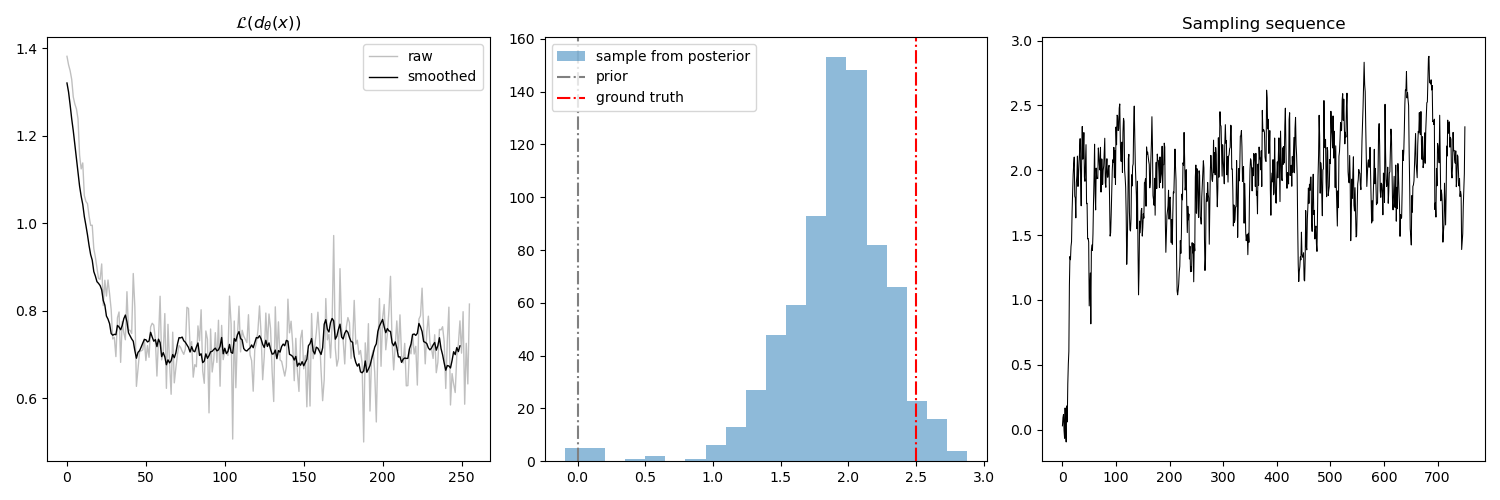
Simulation Based Inference Imagine we have some black-box machine; such a machine has some knobs and levels so we can change its inner configurations. The machine churns out some data for each configuration. The Simulation-based inference (SBI) solves the inverse problem that is given some data, estimating the configuration (Frequentist approach) or sampling the configuration from the posterior distribution (for Bayesian approach). For a formal definition and review of current methods for SBI, see this paper....

TLDR The paper proposed a method to estimate the probability density function of a dataset by discriminating observed data and noise drawn from a distribution. The paper setups the problem into a dataset of \(T\) observations \((x_1, … x_T)\) drawn from a true distribution \(p_d(.)\). We then try to approximate \(p_d\) by a parameterized function \(p_m(.;\theta)\). The estimator \(\hat{\theta}_T\) is defined to be the \(\theta\) that maximize function $$ J_T(\theta) = \frac{1}{2T}\sum_t{\log[h(x_t; 0)]} + \log[1-h(y_t; \theta)] $$...