Surveying numerical methods (finite difference methods) and physics-informed neural networks to solve a 1D heat equation. This post was heavily inspired by:
- (Book) Partial Differential Equations for Scientists and Engineers - Standley J. Farlow for deriving closed-form solution.
- (Article) Finite-Difference Approximations to the Heat Equation
- (Course) ETH Zurich | Deep Learning for Scientific Computing 2023 for Theory and Implementation of Physics-Informed Neural Network.
Introduction
Physics-Informed Machine Learning (PIML) is an exciting subfield of Machine Learning that aims to incorporate physical laws and/or constraints into statistical machine learning. The representations of the laws and constraints can be categorized into three groups (with decreasing strength of inductive bias):
- Partial differential equations (PDE)
- Symmetry: translation, rotation invariant.
- And intuitive physical constraints.
The PINN method incorporates PDE into the learning problem by adding PDE as a regularization term into the machine learning loss term.
Heat equations
This instance of the 1D heat equation describes how the temperature of an insulated rod changes over time (transient state) at any point on the rod, where the two ends of the rod are kept at a constant temperature of \(0^o C\) and the initial temperature of the rod was given by a function of location \(x\).
$$ \begin{equation} \begin{aligned} PDE: & & u_t = \alpha^2 u_{xx} & & 0 < x< 1 & & 0 < t < \infty \\ BCs: & & \begin{cases} u(0, t) = 0\\ u(1, t) = 0 \end{cases} & & 0 < t < \infty \\ IC: & & u(x, 0) = \sin(2\pi x) & & 0 \leq x \leq 1 \end{aligned} \end{equation} $$
Solving heat equation with variables seperation
Suppose that we can factorize \(u(x, t) = X(x)T(t)\), from the PDE we have:
$$ \begin{equation} \begin{aligned} & X(x)T^\prime(t) = \alpha^2 X^{\prime\prime}(x)T(t)\\ \implies & \frac{T^\prime(t)}{\alpha^2 T(t)} = \frac{X^{\prime\prime}(x)}{X(x)} = \mu \\ \implies & \begin{cases} T^\prime(t) - \mu\alpha^2 T(t) = 0 & & (2a) \\ X^{\prime\prime}(x) - \mu X(x) = 0 & & (2b) \end{cases} \end{aligned} \end{equation} $$
From equation (2a), \(T(t) = Ae^{\mu\alpha^2t}\). This implies \(\mu\) must be negative so that \(T\) doesn’t go to \(\infty\). Let \(\mu = -\lambda^2\), so \(T(t) = Ae^{-\lambda^2\alpha^2t}\). Replacing into (2), we have:
$$ \begin{equation} \begin{aligned} & X^{\prime\prime}(x) + \lambda^2 X(x) = 0 \\ \implies & X(x) = B \sin\lambda x + C\cos\lambda x \end{aligned} \end{equation} $$
Substitute \(T(t), X(x)\) into \(u(x, t)\):
$$ \begin{equation} u(x, t) = e^{-\lambda^2\alpha^2 t}(A\sin\lambda x + B\cos\lambda x) \end{equation} $$
Subsititute this into boundary conditions:
$$ \begin{equation} \begin{aligned} & \begin{cases} u(0, t) = 0 \\ u(1, t) = 0 \end{cases} \\ \implies & \begin{cases} e^{-\lambda^2\alpha^2 t}(A \sin 0 + B \cos 0)= 0 \\ e^{-\lambda^2\alpha^2 t}(A \sin \lambda + B \cos \lambda) = 0 \\ \end{cases}\\ \implies & \begin{cases} B = 0 \\ \lambda = n\pi & n = 1, 2, \cdots \end{cases} \end{aligned} \end{equation} $$
So for a given \(n\), we have a particular solution for \(u(x, t)\):
$$ \begin{equation} u_n(x, t) = A_n e^{-n^2\pi^2\alpha^2 t} \sin n\pi x \end{equation} $$
And the general solution for \(u(x, t)\):
$$ \begin{equation} u(x, t) = \sum_{n=1}^\infty{A}_n e^{-n^2\pi^2\alpha^2t} \sin n\pi x \end{equation} $$
Where \(A_n\) is given by:
$$ \begin{equation} A_n = 2\int_0^1 \sin 2\pi x\sin n\pi x dx = \begin{cases} 0 \quad \text{if }n \neq 2\\ 1 \quad \text{if }n = 2 \end{cases} \end{equation} $$
Finally, we have the solution to the PDE:
$$ \begin{equation} \blue{u(x, t) = e^{-4\pi^2\alpha^2t}\sin 2\pi x} \end{equation} $$
Finite Difference Method
Numerical approximation of first and second order derivative
First Order Forward Difference
Consider a Taylor series expansion of \(\phi(x)\) about point \(x_i\):
$$ \begin{equation} \begin{aligned} & \phi(x_i + \delta x) = \phi(x_i) + \frac{\partial \phi}{\partial x}\bigg\vert_{x_i} \delta x + \frac{\partial^2 \phi}{\partial x^2}\bigg\vert_{x_i} \frac{\delta x^2}{2!} + \frac{\partial^3 \phi}{\partial x^3}\bigg\vert_{x_i} \frac{\delta x^3}{3!} + \cdots \\ \end{aligned} \end{equation} $$
Replace \(\delta x = \Delta x \ll 1\) in equation (10):
$$ \begin{aligned} & \phi(x_i + \delta x) = \phi(x_i) + \frac{\partial \phi}{\partial x}\bigg\vert_{x_i} \Delta x + \frac{\partial^2 \phi}{\partial x^2}\bigg\vert_{x_i} \frac{\Delta x^2}{2!} + \frac{\partial^3 \phi}{\partial x^3}\bigg\vert_{x_i} \frac{\Delta x^3}{3!} + \cdots \\ \implies & \frac{\partial \phi}{\partial x}\bigg\vert_{x_i} = \frac{\phi(x_i +\Delta x) - \phi(x_i)}{\Delta x} \red{\underbrace{ - \frac{\partial^2 \phi}{\partial x^2}\bigg\vert_{x_i} \frac{\Delta x}{2!} - \frac{\partial^3 \phi}{\partial x^3}\bigg\vert_{x_i} \frac{\Delta x^2}{3!} - \cdots }_{\text{Truncation error: }\mathcal{O}(\Delta x)}}\\ & \blue{\approx \frac{\phi(x_i +\Delta x) - \phi(x_i)}{\Delta x}} \end{aligned} $$
Note that in this tutorial, the truncation error is \(\mathcal{O}(\Delta x^2)\). I haven’t been able to understand why yet!!!.
First Order Backward Difference
Replace \(\delta x = -\Delta x, \Delta x \ll 1\) in equation (10):
$$ \begin{equation} \begin{aligned} & \phi(x_i + \delta x) = \phi(x_i) - \frac{\partial \phi}{\partial x}\bigg\vert_{x_i} \Delta x + \frac{\partial^2 \phi}{\partial x^2}\bigg\vert_{x_i} \frac{\Delta x^2}{2!} - \frac{\partial^3 \phi}{\partial x^3}\bigg\vert_{x_i} \frac{\Delta x^3}{3!} + \cdots \\ \implies & \frac{\partial \phi}{\partial x}\bigg\vert_{x_i} = \frac{\phi(x_i) - \phi(x_i - \Delta x)}{\Delta x} \red{\underbrace{ + \frac{\partial^2 \phi}{\partial x^2}\bigg\vert_{x_i} \frac{\Delta x}{2!} - \frac{\partial^3 \phi}{\partial x^3}\bigg\vert_{x_i} \frac{\Delta x^2}{3!} + \cdots }_{\text{Truncation error: }\mathcal{O}(\Delta x)}}\\ & \blue{\approx \frac{\phi(x_i) - \phi(x_i - \Delta x)}{\Delta x}} \end{aligned} \end{equation} $$
Second Order Central Difference
Replace in equation (10):
- \(\delta x = \Delta x\)
$$ \begin{equation} \begin{aligned} & \phi(x_i + \Delta x) = \phi(x_i) + \frac{\partial \phi}{\partial x}\bigg\vert_{x_i} \Delta x + \frac{\partial^2 \phi}{\partial x^2}\bigg\vert_{x_i} \frac{\Delta x^2}{2!} + \frac{\partial^3 \phi}{\partial x^3}\bigg\vert_{x_i} \frac{\Delta x^3}{3!} + \cdots \end{aligned} \end{equation} $$
- \(\delta x = -\Delta x\)
$$ \begin{equation} \begin{aligned} & \phi(x_i - \Delta x) = \phi(x_i) - \frac{\partial \phi}{\partial x}\bigg\vert_{x_i} \Delta x + \frac{\partial^2 \phi}{\partial x^2}\bigg\vert_{x_i} \frac{\Delta x^2}{2!} - \frac{\partial^3 \phi}{\partial x^3}\bigg\vert_{x_i} \frac{\Delta x^3}{3!} + \cdots \end{aligned} \end{equation} $$
Adding equation (12) and (13) we have:
$$ \begin{equation} \begin{aligned} & \phi(x_i + \Delta x) + \phi(x_i - \Delta x) = 2 \phi(x_i) + 2 \frac{\partial^2 \phi}{\partial x^2}\bigg\vert_{x_i} \frac{\Delta x^2}{2!} + 2 \frac{\partial^4 \phi}{\partial x^4}\bigg\vert_{x_i} \frac{\Delta x^4}{4!} + \cdots\\ \implies & \frac{\partial^2 \phi}{\partial x^2}\bigg\vert_{x_i} = \frac{\phi(x_i + \Delta x) - 2\phi(x_i) + \phi(x - \Delta x)}{\Delta x^2} \red{\underbrace{ - 2 \frac{\partial^4 \phi}{\partial x^4}\bigg\vert_{x_i} \frac{\Delta x^2}{4!} - \cdots}_{\mathcal{O}(\Delta x^2)}}\\ & \blue{ \approx \frac{\phi(x_i + \Delta x) - 2\phi(x_i) + \phi(x - \Delta x)}{\Delta x^2} } \end{aligned} \end{equation} $$
Finite Difference Method for the Heat Equation
Discretize the domain \(\mathcal{D} = (0, 1) \times (0, T)\) by constructing a grid \(\{x_i\}_{i=1\cdots N} \times \{t_m\}_{m=1\cdots M}\). Where:
- \(x_i = (i - 1) \Delta x,\quad \Delta x = \frac{1}{N - 1}\)
- \(t_m = (m - 1) \Delta t,\quad \Delta t = \frac{T}{M - 1}\)
Let \(u(x, t)\) be the true solution to the PDE
Forward Time, Centered Space (FTCS)
Using First Order Forward Difference (equation 10) to approximate parital derivative of \(u\) at a grid point \((x_i, t_m)\):
$$ \begin{equation} \begin{aligned} \frac{\partial u}{\partial t} \bigg\vert_{x=x_i, t=t_m} & = \frac{u(x_i, t_m + \Delta t) - u(x_i, t_m)}{\Delta t} + \mathcal{O}(\Delta t)\\ & \approx \frac{u_i^{m+1}-u_i^m}{\Delta t} \end{aligned} \end{equation} $$
Using Second Order Central Difference (equation 14) to approximate the second order partial derivative of \(u\) with respect to \(x\) at the grid point: $$ \begin{equation} \begin{aligned} \frac{\partial^2 u}{\partial x^2} \bigg\vert_{x=x_i, t=t_m} & = \frac{u(x_i + \Delta x, t_m) - 2 u(x_i, t_m) + u(x_i - \Delta x, t_m)}{\Delta x^2} + \mathcal{O}(\Delta x^2)\\ & \approx \frac{u_{i+1}^m - 2 u_i^m + u_{i-1}^m}{\Delta x^2} \end{aligned} \end{equation} $$
Where \(u_i^m\) is the numerical approximation of true function evaluated at the grid point \((x_i, t_m)\). Replacing equation (15) and (16) into the LHS and RHS of the PDE in (1):
$$ \begin{equation} \begin{aligned} & \frac{u_i^{m+1}-u_i^m}{\Delta t} = \alpha^2 \frac{u_{i+1}^m - 2 u_i^m + u_{i-1}^m}{\Delta x^2}\\ \implies & u_i^{m+1} = u_i^m + \frac{\alpha^2 \Delta t}{\Delta x^2} (u_{i+1}^m - 2 u_i^m + u_{i-1}^m) \\ & = \blue{u_i^m(1 - 2r) + r(u_{i+1}^m + u_{i-1}^m)} \end{aligned} \end{equation} $$
Where \(r = \frac{\alpha^2\Delta t}{\Delta x^2}\). In order for \(u(x, t)\) reach steady state, \(r\) must be smaller than \(\frac{1}{2}\). The proof was provided in Von Neumann Stability Analysis.
TODO: Haven’t understood yet !!!
Equation (17) allows us to sequentially compute the approximation \(u_i^m\) at any point \((x_i, t_m)\), where \(u_i^1 = u(x_i, 0), i = 1\cdots N\) were given by the initial and boundary conditions. In matrix notation, the series of equation can be written as:
$$ \begin{equation} \begin{aligned} \begin{bmatrix} 1 & 0 & 0 & 0 & 0 & 0 & 0 \\ r & 1 - 2r & r & \cdots & 0 & 0 & 0 \\ \vdots & \vdots &\vdots &\ddots &\vdots &\vdots &\vdots \\ 0 &0 & 0 & \cdots & r & 1 - 2r & r \\ 0 & 0 & 0 & 0 & 0 & 0 & 1 \end{bmatrix} \underbrace{\begin{bmatrix} u_1^m \\ u_2^m \\ \vdots \\ u_{N-1}^m \\ u_N^m \\ \end{bmatrix}}_{u^m} = \underbrace{\begin{bmatrix} u_1^{m+1} \\ u_2^{m+1} \\ \vdots \\ u_{N-1}^{m+1} \\ u_N^{m+1} \\ \end{bmatrix}}_{u^{m+1}} \end{aligned} \end{equation} $$
Note that \(u_1^m\), \(u_N^m\) are always equal to its value in the next time step. This is due to the boundary condition, the temperature at the boundary is always \(0\).
(code) Implementation of FTCS scheme
solve_fdm() 1
2
3
4
5
6
7
8
9
10
11
12
13
14
15
16
17
18
19
20
21
22
23
24
25
26
27
28
29
30
31
32
33
34
35
36
37
38
39
40
41
42
import numpy as np


def solve_fdm(N: int, M: int, T: float):
    """
    solving 1D heat equation:
        PDE: u_t = u_xx (\alpha^2 = 1)
        BCs: u(0, t) = u(1, t) = 0
        ICs: u(x, 0) = x - x**2

    args:
        - N, M  : number of collocation points
            in spacial and temporal dimension
        - T     : solving from t = 0 to T
    """

    # constructing the grid
    dx = 1 / (N - 1) # 0 <= x <= 1
    dt = T / (M - 1) # 0 < t <= T

    r = dt/dx**2 # (alpha = 1)

    # Condition for numerical stability
    assert r < .5, ValueError(f"Choose smaller r, r={r:.4f}")

    x_grid = np.linspace(0, 1, N)

    # approximate the result
    U = np.zeros((N, M)) # already satisfied the BCs

    # IC impose initial condition
    ic = lambda x: np.sin(2 * np.pi * x)
    U[:, 0] = np.vectorize(ic)(x_grid)

    # kernel to approximate 2nd derivative of u wrt x
    ker = np.array([1., -2., 1.], dtype=np.float64)

    for i in range(1, M):
        ut = np.convolve(U[:, i - 1], ker, mode="same")
        U[:,i] = U[:, i-1] + r * ut

    return U
| |
 |  |
Backward Time, Centered Space (BTCS)
Using First Order Backward Difference (equation 11) to approximate parital derivative of \(u\) at a grid point \((x_i, t_m)\):
$$ \begin{equation} \begin{aligned} \frac{\partial u}{\partial t} \bigg\vert_{x=x_i, t=t_m} & = \frac{u(x_i, t_m) - u(x_i, t_m - \Delta t)}{\Delta t} + \mathcal{O}(\Delta t)\\ & \approx \frac{u_i^{m}-u_i^{m-1}}{\Delta t} \end{aligned} \end{equation} $$
Using Second Order Central Difference (equation 14) to approximate the second order partial derivative of \(u\) with respect to \(x\) at the grid point: $$ \begin{equation} \begin{aligned} \frac{\partial^2 u}{\partial x^2} \bigg\vert_{x=x_i, t=t_m} & = \frac{u(x_i + \Delta x, t_m) - 2 u(x_i, t_m) + u(x_i - \Delta x, t_m)}{\Delta x^2} + \mathcal{O}(\Delta x^2)\\ & \approx \frac{u_{i+1}^m - 2 u_i^m + u_{i-1}^m}{\Delta x^2} \end{aligned} \end{equation} $$
Replacing equation (19), and (20) into LHS and RHS of the PDE in (1) respectively we have:
$$ \begin{equation} \begin{aligned} & \frac{u_i^{m}-u_i^{m-1}}{\Delta t} = \alpha^2 \frac{u_{i+1}^m - 2 u_i^m + u_{i-1}^m}{\Delta x^2}\\ \implies & u_i^{m-1} = u_i^m - \frac{\alpha^2 \Delta t}{\Delta x^2} (u_{i+1}^m - 2 u_i^m + u_{i-1}^m) \\ & = \blue{u_i^m(1 + 2r) - r(u_{i+1}^m + u_{i-1}^m)} \end{aligned} \end{equation} $$
Where \(r = \frac{\alpha^2\Delta t}{\Delta x^2}\). Rewriting equation(21) in matrix notation:
$$ \begin{equation} \begin{aligned} \underbrace{\begin{bmatrix} 1 & 0 & 0 & 0 & 0 & 0 & 0 \\ -r & 1 + 2r & -r & \cdots & 0 & 0 & 0 \\ \vdots & \vdots &\vdots &\ddots &\vdots &\vdots &\vdots \\ 0 &0 & 0 & \cdots & -r & 1 + 2r & -r \\ 0 & 0 & 0 & 0 & 0 & 0 & 1 \end{bmatrix}}_A \underbrace{\begin{bmatrix} u_1^m \\ u_2^m \\ \vdots \\ u_{N-1}^m \\ u_N^m \\ \end{bmatrix}}_{\mathbf{u}^m} = \underbrace{\begin{bmatrix} u_1^{m-1} \\ u_2^{m-1} \\ \vdots \\ u_{N-1}^{m-1} \\ u_N^{m-1} \\ \end{bmatrix}}_{\mathbf{u}^{m-1}} \end{aligned} \end{equation} $$
So that we can sequentially compute the next state by solving the system of linear equations in (22):
$$ \blue{ \mathbf{u}^{m} = A^{-1} \mathbf{u}^{m-1}; \quad m = 2,\cdots M } $$
Where \(\mathbf{u}_i^1\) are given by the initial and boundary conditions. Unlike FTCS, BTCS are unconditionally stable with respect to the choice of \(r\). Therefore we can choose much fewer steps along temporal dimension.
(code) Implementation of BTCS scheme
solve_bdm() 1
2
3
4
5
6
7
8
9
10
11
12
13
14
15
16
17
18
19
20
21
22
23
24
25
26
27
28
29
30
31
32
33
34
35
36
37
38
39
40
41
42
import numpy as np
from scipy.sparse import diags

def solve_bdm(N: int, M: int, T: float):
    """
    solving 1D heat equation using BTCS scheme
        PDE: u_t = u_xx (\alpha^2 = 1)
        BCs: u(0, t) = u(1, t) = 0
        ICs: u(x, 0) = x - x**2

    args:
        - N, M  : number of collocation points
            in spacial and temporal dimension
        - T     : solving from t = 0 to T
    """
    # constructing the grid
    dx = 1 / (N - 1) # 0 <= x <= 1
    dt = T / (M - 1) # 0 < t <= T

    r = dt/dx**2 # (alpha = 1)

    # construct A:
    A = diags([-r, 1 + 2 * r, -r], [-1, 0, 1], shape=(N, N)).toarray()
    A[0, :] = 0
    A[-1, :] = 0
    A[0, 0] = 1
    A[-1,-1] = 1

    A_inv = np.linalg.inv(A)

    # approximate the result
    U = np.zeros((N, M)) # already satisfied the BCs

    # IC impose initial condition
    x_grid = np.linspace(0, 1, N)
    ic = lambda x: np.sin(2 * np.pi * x)
    U[:, 0] = np.vectorize(ic)(x_grid)

    for m in range(1, M):
        U[:, m] = A_inv @ U[:, m-1]

    return U
| |
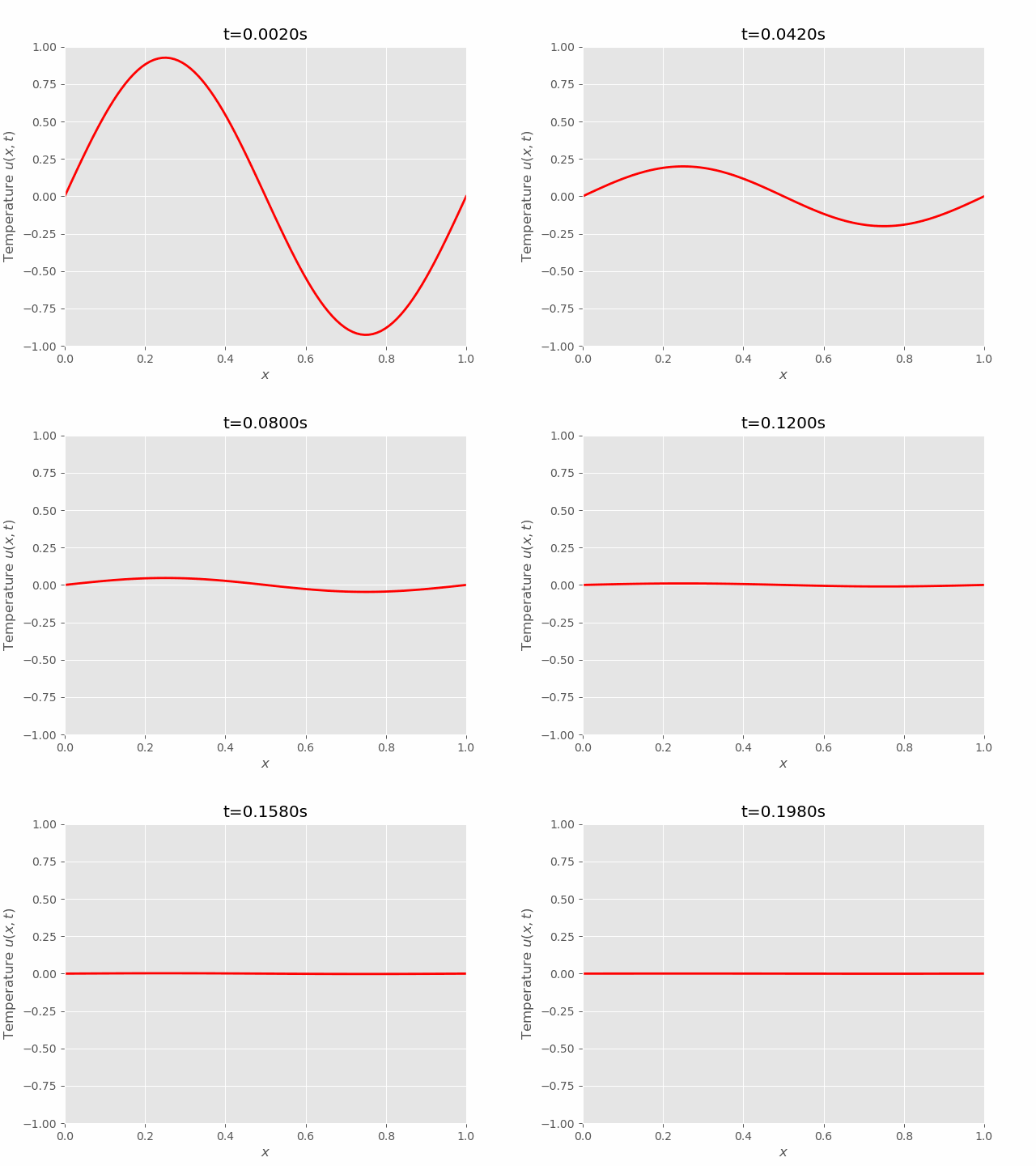 | 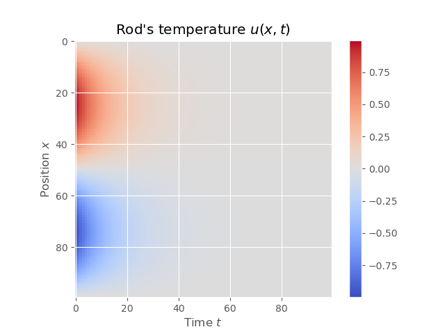 |
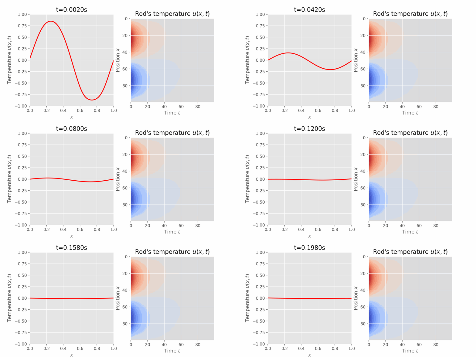
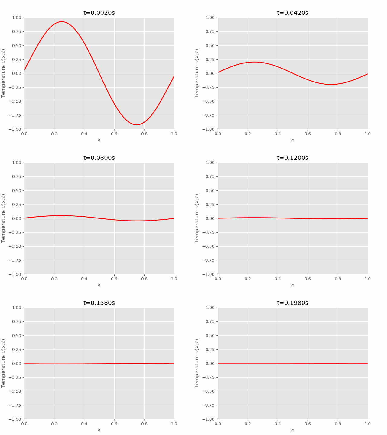
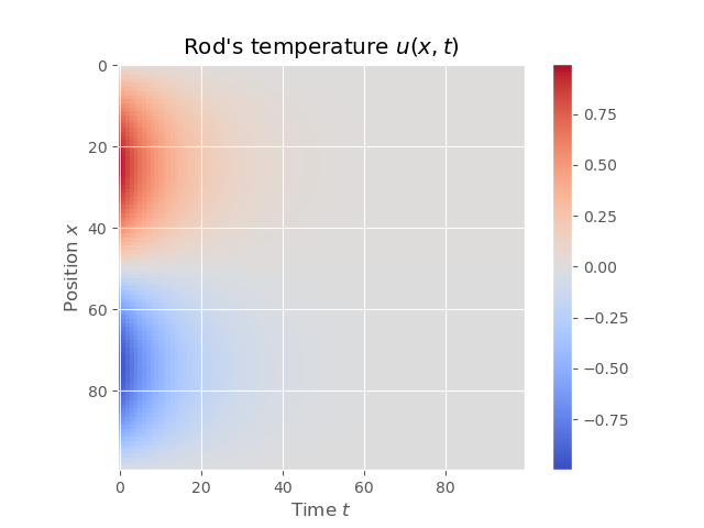
We can see that results of FTCS and BTCS agree with each other, however, BTCS only using a \(100 \times 100\) grid while FTCS using \(100 \times 4000\) grid.
There is one more scheme for finite different methods which is Crank-Nicolson methods, which use central diffence method to estimate first order derivative !!
Physics Informed Neural Network
Let’s rewrite the heat equation in a more general form:
$$ \begin{equation} \begin{aligned} PDE: & & u_t = \alpha^2 u_{xx} & & 0 < x< 1 & & 0 < t < \infty \\ BCs: & & \begin{cases} u(0, t) = f_0(t)\\ u(1, t) = f_1(t) \end{cases} & & 0 < t < \infty \\ IC: & & u(x, 0) = \phi(t) & & 0 \leq x \leq 1 \end{aligned} \end{equation} $$
In our case, \(f_0(t) = f_1(t) = 0\) and \(\phi(x) = \sin 2\pi x\). PINN approximate the function \(u(x, t)\) by a neural network \(U_\theta(x, t)\), and then learn the networks parameters \(\theta\) by minimize the loss function:
$$ \begin{equation} \begin{aligned} \mathcal{L}(\theta) & = \frac{1}{N}\sum_{i=1}^N{[U_\theta(x_i, t_i) - u_i]^2} & \text{(Supervised loss)}\\ & + \frac{\lambda_j}{M_j} \sum_{j=1}^{M_j}{\bigg[ \frac{\partial U_\theta}{\partial t}- \alpha^2 \frac{\partial^2 U_\theta}{\partial x^2} \bigg](x_j, t_j)} & \text{(PDE residual)}\\ & + \frac{\lambda_k}{M_k} \sum_{k=1}^{M_k}{[(U_\theta(0, t_k) - f_0(t_k))^2 + (U_\theta(1, t_k) - f_1(t_k))^2]} & \text{(Boundary conditions)} \\ & + \frac{\lambda_h}{M_h} \sum_{h=1}^{M_h}{[U_\theta(x_h, 0) - \phi(x_h)]^2} & \text{(Initial condition)} \end{aligned} \end{equation} $$
The first term is the supervised loss, coinciding with statistical machine learning. Where \({(x_i, t_i, u_i)}_{i=1\cdots N}\) is the set of collocation points \((x_i, t_i)\), and value of \(u_i = u(x_i, t_i)\).
The second term is the PDE residual, where:
- \(\frac{\partial U_\theta}{\partial t}\) is the partial derivative of the network \(U_\theta\) with respect to the time input \(t\)
- Similarly, \(\frac{\partial^2 U_\theta}{\partial x^2}\) is the second derivative of the network with repsect to location \(x\).
Second and third terms are the initial and boundary conditions, given by equation (23).
We don’t necessarily have access to the first loss term. In the implementation bellow, I ignored the first loss term. For the remaining three loss terms:
- PDE residual: \(x_j \sim \text{Uniform}(0, 1); t_j \sim\text{Uniform}(0, 0.2)\)
- Boundary condition: \(t_k \sim \text{Uniform}(0, 0.2)\)
- Initial condition: \(x_h \sim \text{Uniform}(0, 1)\)
Note: The code need some refactoring but it still works.
(code) JAX Implementation of PINN:
train(), and compute_grid() 1
2
3
4
5
6
7
8
9
10
11
12
13
14
15
16
17
18
19
20
21
22
23
24
25
26
27
28
29
30
31
32
33
34
35
36
37
38
39
40
41
42
43
44
45
46
47
48
49
50
51
52
53
54
55
56
57
58
59
60
61
62
63
64
65
66
67
68
69
70
71
72
73
74
75
76
77
78
79
80
81
82
83
84
85
86
87
88
89
90
91
92
93
94
95
96
97
98
99
100
101
102
103
104
105
106
107
108
109
110
111
112
113
114
115
116
117
118
119
120
121
122
123
124
125
126
127
128
129
130
131
132
133
134
135
136
137
138
139
140
141
142
143
144
145
146
147
148
149
150
151
152
153
154
155
156
157
158
159
160
161
162
163
164
165
166
167
168
169
170
171
172
173
174
175
176
177
178
179
180
181
182
183
184
185
186
187
188
189
190
191
192
193
194
195
196
197
198
199
200
201
202
203
204
205
206
207
208
209
210
211
212
213
214
215
216
217
218
import numpy as np
import click
import equinox as eqx
import jax
import jax.numpy as jnp
import optax
import yaml
from matplotlib import pyplot as plt
from pydantic import BaseModel
from pydantic import PositiveInt
from tqdm import trange
from src.viz import plot_heatmap
from src.viz import animate


# Plot config
plt.style.use('ggplot')


class PINNConfig(BaseModel):
    key: int
    layers: list[PositiveInt]
    batch_ic_size: PositiveInt
    batch_bc_size: PositiveInt
    batch_interior_size: PositiveInt
    fn_path: str
    fn_path_gif: str


class U(eqx.Module):
    """
    Simple MLP taking (x, t) as input, return mlp(x, t)
    """

    layers: list #

    def __init__(self, layers: list[int], key):
        self.layers = []

        for _in, _out in zip(layers[:-1], layers[1:]):
            key, subkey = jax.random.split(key, 2)
            self.layers.append(eqx.nn.Linear(_in, _out, key=subkey))

    def __call__(self, x, t):
        """
        assuming x in R^{n x (d - 1)}, t in R
        """
        out = jnp.concatenate([x, t], axis=-1)

        for layer in self.layers[:-1]:
            out = layer(out)
            out = jax.nn.tanh(out)

        out = self.layers[-1](out)
        return jax.nn.tanh(out)


def interior_loss(u, x, t):
    """
    """
    # First and second derivative of u wrt x
    u_x = jax.grad(lambda x, t: jnp.squeeze(u(x, t)), argnums=0)
    u_xx = jax.grad(lambda x, t: jnp.squeeze(u_x(x, t)), argnums=0)
    u_t = jax.grad(lambda x, t: jnp.squeeze(u(x, t)), argnums=1)

    pde_resid = jax.vmap(u_t)(x, t) - jax.vmap(u_xx)(x, t)
    return jnp.mean(pde_resid**2)


def boundary_loss(u, x, t, f_bc: callable):
    """
    """
    # compute boundary value at each collocation point
    y = jax.vmap(f_bc)(x, t)
    y_hat = jax.vmap(u)(x, t)

    return jnp.mean((y - y_hat) ** 2)


def initial_condition_loss(u, x, t, f_ic):
    y = jax.vmap(f_ic)(x, t)
    y_hat = jax.vmap(u)(x, t)

    return jnp.mean((y - y_hat) ** 2)


def generate_interior_batch(key, n):
    """
    interior collocation points
    """
    # sample, discretizing interior point
    key, subkey = jax.random.split(key, 2)
    X = jax.random.uniform(subkey, shape=(n, 1), minval=1e-5, maxval=1-1e-5)

    key, subkey = jax.random.split(key, 2)
    T = jax.random.uniform(subkey, shape=(n, 1), minval=1e-5, maxval=.2)

    return X, T

def generate_ic_batch(key, n):
    """
    initial collocation points {(x_i, 0)}
    """
    # sample, discretizing interior point
    key, subkey = jax.random.split(key, 2)
    X = jax.random.uniform(subkey, shape=(n, 1), minval=1e-5, maxval=1-1e-5)

    key, subkey = jax.random.split(key, 2)
    T = jnp.zeros(shape=(n, 1))

    return X, T

def generate_bc_batch(key, n):
    """
    initial collocation points {(0/1, t_m)}
    """
    # sample, discretizing interior point
    key, subkey = jax.random.split(key, 2)
    X = jax.random.randint(subkey, shape=(n, 1), minval=0., maxval=2.)

    key, subkey = jax.random.split(key, 2)
    T = jax.random.uniform(subkey, shape=(n, 1), minval=1e-5, maxval=.2)

    return X, T


def loss_fn(u, x_i, t_i, x_ic, t_ic, x_bc, t_bc, f_ic, f_bc):
    """
    u: model
    x_i, t_i: interior collocation point
    x_ic, t_ic: initial points
    x_bc, t_bc: boundar points
    f_ic: initial condition
    f_bc: boundary condition
    """
    return interior_loss(u, x_i, t_i) +\
            initial_condition_loss(u, x_ic, t_ic, f_ic) +\
            boundary_loss(u, x_bc, t_bc, f_bc)


def train(config: PINNConfig):
    key = jax.random.PRNGKey(config.key)
    key, subkey = jax.random.split(key, 2)

    # define the model
    u = U(config.layers, subkey)

    # define initial condition
    def f_ic(x, t):
        return jnp.sin(2 * jnp.pi * x)

    # define boundary condition
    def f_bc(x, t):
        return 0.

    # compute loss & loss gradient
    grad_loss_fn = jax.value_and_grad(loss_fn)

    @jax.jit
    def train_step(model, key, optim_state):
        # Generate data point
        ic_key, bc_key, i_key = jax.random.split(key, 3)
        x_ic, t_ic = generate_ic_batch(ic_key, config.batch_ic_size)
        x_bc, t_bc = generate_bc_batch(bc_key, config.batch_bc_size)
        x_i, t_i = generate_interior_batch(i_key, config.batch_interior_size)

        loss_val, grads = grad_loss_fn(
                model, x_i, t_i,
                x_ic, t_ic,
                x_bc, t_bc,
                f_ic, f_bc)
        updates, optim_state = optim.update(grads, optim_state)
        new_model = eqx.apply_updates(model, updates)

        return loss_val, new_model, key, optim_state

    # optimizer
    optim = optax.adam(1e-3)
    optim_state = optim.init(u)

    losses = []
    pbar = trange(10000)

    for i in pbar:
        loss, u, key, optim_state = train_step(u, key, optim_state)
        pbar.set_description(f"Loss = {loss:.4f}")
        losses.append(loss)

    losses = jnp.array(losses)

    return u, losses


def compute_grid(model: eqx.Module, config: PINNConfig):
    """
    compute model output on 100 x 100 grid over following domain
    x in (0, 1)
    t in (0, 0.2)
    """

    def _compute(x, t):
        # transform scalar into a 1d vector x -> [x]
        x, t = jnp.expand_dims(x, 0),\
                jnp.expand_dims(t, 0)

        u = model(x, t)
        u = jnp.squeeze(u)

        return u

    x = jnp.linspace(0, 1, 100)
    t = jnp.linspace(0, 0.2, 100)

    xx, tt = np.meshgrid(x, t, sparse=True)
    U = np.vectorize(_compute)(xx, tt).T

    return U
| |
