todo
- Derivation of second and forth order Runge-Kutta methods
- Comparison of truncation error with different step-size
Ordinary Differential Equation (ODE) Initial Value Problem
A differential equation is differential equation is a relationship between function \(f(x)\), its independent variable \(x\), and any number of its derivative. An ODE is a differential equation where the independent variable and its derivatives are in one dimension.
$$ \begin{equation} F(x, f(x), f^{(1)}(x), f^{(2)}, \cdots f^{(n-1)}(x)) = f^{(n)}(x) \end{equation} $$
Where \(f^{(i)}\) is the \(i^{th}\) order derivative of \(f\). Initial value is a set of known value at \(x = 0\), namely \(f(0), f^{(1)}(0), f^{(2)}, \cdots f^{(n-1)}(0)\). Coupled with equation 1, the problem is known as the ODE Initial Value Problem.
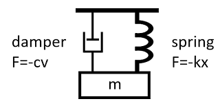
An example is the dampen harmonic occillator with the setup as following diagram:

The motion of mass \(m\) is gorverned by set of equations:
$$ \begin{equation} \begin{aligned} ODE \quad & F(t, x, \dot{x}) = -\frac{c \dot{(x)} + kx}{m} = \ddot{x} \\ IV \quad & x(0) = A\\ & \dot{x}(0) = 0 \end{aligned} \end{equation} $$
Reduction or Order
Denote \(S(x)\) to be a state of equation (1):
$$ \begin{equation} \begin{aligned} & S(x) = \begin{bmatrix} f(x) \\ f^{(1)}(x) \\ \vdots \\ f^{(n-1)}(x) \\ \end{bmatrix} \\ \end{aligned} \end{equation} $$
So equation 1 can be rewriten as
$$ \begin{equation} \begin{aligned} F(t, S(t)) = f^{(n)}(t) \end{aligned} \end{equation} $$
Taking derivative of \(S\)
$$ \begin{equation} \begin{aligned} & \frac{dS}{dt} = \begin{bmatrix} f^{(1)}(x) \\ f^{(2)}(x) \\ \vdots \\ f^{(n)}(x) \\ \end{bmatrix} = \begin{bmatrix} S_2(x) \\ S_3(x) \\ \vdots \\ F\big(x, S(t)) \end{bmatrix} & \text{(Equation 3)} \\ & = \mathcal{F}(t, S(t)) \end{aligned} \end{equation} $$
Where \(S_i(x)\) is the \(i^{th}\) entry of \(S(x)\). The \(n^{th}\) order ODE is turned into \(n\) coupled ODEs, where \(\mathcal{F}\) is a function that assemble the correct state vector.
Back to the dampend harmonic occilliator, we can denote the state vector \(S(t)\) as:
$$ \begin{equation} \begin{aligned} & S(t) = \begin{bmatrix} x(t)\\ \dot{x}(t) \end{bmatrix} \\ \implies & \frac{dS}{dt} = \begin{bmatrix} \dot{x}(t)\\ \ddot{x}(t) \end{bmatrix} \\ & = \begin{bmatrix} S_2(t)\\ F(t, x, \dot{x}) \end{bmatrix} & \text{(ODE in 2)} \\ & = \begin{bmatrix} 0 & 1 \\ -k/m & -c/m \end{bmatrix} \begin{bmatrix} x(t)\\ \dot{x}(t) \end{bmatrix} \\ & = \begin{bmatrix} 0 & 1 \\ -k/m & -c/m \end{bmatrix}S(t) \end{aligned} \end{equation} $$
So the second order ODE describes motion of mass \(m\) is transformed into a first order ODE of the state \(S(t)\).
Numerical methods of solving first order ODE
Given the formulation \(\frac{dS}{dt} = \mathcal{F}(t, S(t))\), and a regular grid on temporal interval \([0, T]: \{t_0, t_1,\cdots t_N\}\), where \(t_i = i\frac{T}{N}=:ih\). The Taylor expansion of \(S\) about \(t\) is given by:
$$ \begin{equation} \begin{aligned} S(t+h) = S(t) + \sum_1^k{ \frac{h^k}{k!} \frac{d^{(k)}S}{dt}(t) } + \mathcal{O}(h^{k+1}) \end{aligned} \end{equation} $$
Euler method
The Euler method approximate the next state by simply truncating the Taylor expansion after the first derivative.
$$ \begin{equation} \begin{aligned} \hat{S}(t_{i+1}) = S(t_i + h) & = S(t_i) + h \frac{dS}{dt}(t_i) + \mathcal{O}(h^2)\\ & = S(t_i) + h\mathcal{F}(t_i, S(t_i)) + \underbrace{\red{\mathcal{O}(h^2)}}_{\text{Truncation Error}} \end{aligned} \end{equation} $$
Given \(\mathcal{F}, S_0\) we can sequentially compute \(S\) at any time \(t\).
(code) JAX Implementation of Euler method
euler() 1
2
3
4
5
6
7
8
9
10
11
12
13
14
15
16
17
18
19
20
21
22
23
def euler(z0: jnp.ndarray, t0: float, t1: float, f: callable,
          return_seq: bool = False):
    n_steps = int(jnp.ceil(jnp.abs(t1 - t0)/H_MAX))

    # Compute step size
    h = (t1 - t0)/n_steps

    t = t0
    z = z0

    # sequence of z
    seq = [(z, t)]

    for i in range(n_steps):
        z = z + h * f(z, t)
        t = t + h

        seq.append((z, t))

    if return_seq:
        return z, seq

    return z
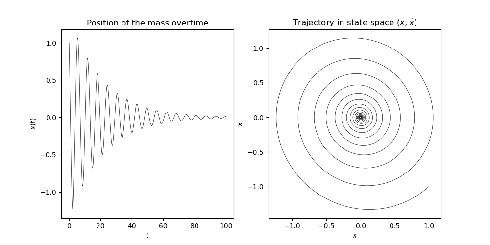
Let’s try this on the dampen harmonic occilliator example with parameters:
| |
(code)
dampen_harmonic_occiliator() 1
2
3
4
5
6
7
8
9
10
11
12
13
14
15
16
17
18
19
20
21
22
23
24
25
26
27
28
29
30
31
32
# Dampen Harmoic Occililator
def dampen_harmonic_occiliator(
        c   : PositiveFloat,
        k   : PositiveFloat,
        m   : PositiveFloat,
        A   : float,
        V   : float,
        t0  : float,
        t1  : float):
    """
    Problem:
        ODE: x'' + c/m x' + k/m x = 0
        IV: x(t0) = A, x'(t0) = V

    Params:
        c: dampener coefficient
        k: spring coefficient
        m: mass
        A, V: initial position and velocity
        t0, t1: start and terminal timestamp
    """

    # constructing dynamic function
    F = lambda S, t: jnp.array([[0, 1],[-k/m, -c/m]]) @ S

    # initial condition
    S = jnp.array([A, V])

    # Terminal S and trajectory of S
    S_t, Tr = euler(S, t0, t1, F, True)

    return S_t, Tr
| |
Results

Runge-Kutta
Second-Order Runge-Kutta Method
Second-Order Runge-Kutta Method reduces the truncation errors in the estmation of the next state to \(\mathcal{O}(h^3)\) by keeping the \(3^{rd}\) term in the Taylor expansion.
$$ \begin{equation} S(t_{i+1}) = S(t_i + h) = S(t_i) + h \mathcal{F}(t_i, S(t_i)) + \underbrace{ \frac{h^2}{2!} \mathcal{F}^\prime(t_i, S(t_i)) }_{A} + \mathcal{O}(h^3) \end{equation} $$
Consider quantity \(A\):
$$ \begin{equation} \begin{aligned} A & = \frac{d}{dt} \mathcal{F}(t, S(t)) = \frac{\partial\mathcal{F}}{\partial t} + \frac{\partial F}{\partial S}\frac{dS}{dt} \\ & = \frac{\partial\mathcal{F}}{\partial t} + \frac{\partial\mathcal{F}}{\partial S} F & \text{(Equation 5)} \end{aligned} \end{equation} $$
Substitute equation 10 into equation 9:
$$ \begin{equation} \begin{aligned} S(t_{i+1}) = S(t_i + h) & = S + h\mathcal{F} \\ & + \frac{h^2}{2}\big( \frac{\partial\mathcal{F}}{\partial t} + \frac{\partial\mathcal{F}}{\partial S}\mathcal{F} \big) \\ &+ \mathcal{O}(h^3) \end{aligned} \end{equation} $$
Consider approximation of \(\mathcal{F}\) in the neighbor of \((t, S\)
$$ \begin{equation} \begin{aligned} \mathcal{F}(t + ph, S + qhF) & = F + \frac{\partial\mathcal{F}}{\partial t}\delta t + \frac{\partial\mathcal{F}}{\partial S} \delta S \\ & = S + \end{aligned} \end{equation} $$
(code) JAX Implementation of Second-Order Runge Kutta method
RK2() 1
2
3
4
5
6
7
8
9
10
11
12
13
14
15
16
17
18
19
20
21
22
23
24
25
26
27
28
29
def RK2(z0, t0, t1, f, return_seq: bool):
    """
    Second-Order Runge-Kutta Method
    S(t + h) = S(t) + 1/2(k1 + k2)h
    k1 = F(t, S(t))
    k2 = F(t + h, S(t) + hk1)
    """
    n_steps = int(jnp.ceil(jnp.abs(t1 - t0)/H_MAX))

    # Compute step size
    h = (t1 - t0)/n_steps

    t = t0
    z = z0

    seq = [(z, t)]

    for i in range(n_steps):
        k1 = f(z, t)
        k2 = f(z + h * k1, t + h)
        z = z + .5 * (k1 + k2) * h
        t = t + h

        seq.append((z, t))

    if return_seq:
        return z, seq

    return z
Fourth-Order Runge-Kutta Method
$$ \begin{equation} \begin{aligned} \hat{S}(t + h) & = S(t) + \frac{h}{6}(k_1 + 2k_2 + 2k_3 + k_4) + \underbrace{\red{\mathcal{O}(h^4)}}_{\text{Truncation error}} \\ \text{Where:}\\ k_1 & = \mathcal{F}(t, S(t)) \\ k_2 & = \mathcal{F}(t + \frac{h}{2}, S(t) + \frac{hk_1}{2}) \\ k_3 & = \mathcal{F}(t + \frac{h}{2}, S(t) + \frac{hk_2}{2} \\ k_4 & = \mathcal{F}(t + h, S(t) + hk_3) \\ \end{aligned} \end{equation} $$
(code) JAX Implementation of Second-Order Runge Kutta method
RK2() 1
2
3
4
5
6
7
8
9
10
11
12
13
14
15
16
17
18
19
20
21
22
23
24
25
26
27
28
29
30
31
32
33
34
def RK4(z0, t0, t1, f, return_seq: bool):
    """
    Fourth-Order Runge-Kutta Method
    S(t + h) = S(t) + 1/2(k1 + k2)h
    k1 = F(t, S(t))
    k2 = F(t + .5h, S(t) + .5 h k1)
    k3 = F(t + .5h, S(t) + .5 h k2)
    k4 = F(t + h, S(t) + h k3)
    """
    n_steps = int(jnp.ceil(jnp.abs(t1 - t0)/H_MAX))

    # Compute step size
    h = (t1 - t0)/n_steps

    t = t0
    z = z0

    seq = [(z, t)]


    for i in range(n_steps):
        k1 = f(z, t)
        k2 = f(z    + .5 * k1 * h, t + .5  *   h)
        k3 = f(z    + .5 * k2 * h, t + .5  *   h)
        k4 = f(z    +      k3 * h, t +         h)

        z = z + (k1 + 2 * k2 + 2 * k3 + k4) * h / 6

        seq.append((z, t))

    if return_seq:
        return z, seq

    return z
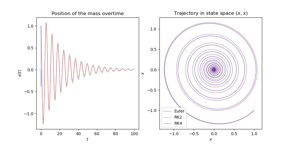
Empirical result
Numerical error by different step-size
Position and Trajectory in state-space

References
- (Book) Partial Differential Equations for Scientists and Engineers - Standley J. Farlow
- (Book) Python Programming and Numerical Methods - A Guide - Chapter 22
- (Web) Introduction to Taylor’s theorem for multivariable functions
- (Web) Analytical solution to Damped Harmonic Occiliator - https://phys.libretexts.org
