Simulation Based Inference
Imagine we have some black-box machine; such a machine has some knobs and levels so we can change its inner configurations. The machine churns out some data for each configuration. The Simulation-based inference (SBI) solves the inverse problem that is given some data, estimating the configuration (Frequentist approach) or sampling the configuration from the posterior distribution (for Bayesian approach). For a formal definition and review of current methods for SBI, see this paper. In the analogy above, the black box represents the simulator, and the configurations are the simulator’s parameters.
The applicability of SBI has great potential since we can almost reduce any process with defined input and output to a black-box machine 1.
This post documents my notes while studying Likelihood-free MCMC with Amortized Ratio Estimator (Hermans et al, 2020); a method developed to address SBI.
Likelihood-free MCMC with Amortized Ratio Estimator
Likelihood ratio is defined as the ratio between the likelihood of the observation between two different hypothesis:
$$ r(\mathbf{x} | \theta_0, \theta_1) = \frac{p(\mathbf{x} | \theta_0)}{p(\mathbf{x}|\theta_1)} $$
This quantity then can be used in various methods to draw sample from a distribution. In the paper, the author mention three sampling methods, namely Markov Chain Monte Carlo, Metropolis-Hasting, and HMC. In the following section, I am briefly summarizing those methods.
Background
Markov Chain Monte Carlo (MCMC)
In statistics, the MCMC method is a class of algorithms for sampling from a probability distribution. By constructing a Markov chain with the desired distribution as its equilibrium distribution, one can obtain a sample of the desired distribution by recording states from the state chain 2.
Adapting MCMC for SBI task
We want to sample from \(p(\theta | \mathbf{x})\) using MCMC, we need this quantity
$$ \begin{equation} \begin{aligned} \frac{p(\theta | \mathbf{x} )}{p(\theta_t| \mathbf{x})} = \frac{ p(\theta)p(\mathbf{x} | \theta)/p(\mathbf{x}) }{ p(\theta_t)p(\mathbf{x} | \theta_t)/p(\mathbf{x}) } = \frac{p(\theta)}{p(\theta_t)}\times \frac{p(\mathbf{x} | \theta)}{p(\mathbf{x} | \theta_t)} = \frac{p(\theta)}{p(\theta_t)} \times r(\mathbf{x} | \theta, \theta_t) \end{aligned} \end{equation} $$
We can compute the first term of the equation since we have access to prior \(p(\theta)\). But we can not compute the second term because we do not have access to the likelihood function \(p(\mathbf{x} | \theta)\). However, we can reframe the problem in the supervised-learning paradigm, so we can use a parameterized discriminator \(d_\theta(\mathbf{x})\) to estimate the likelihood. The details are described in the Likelihood Ratio Estimator section.
Metropolis-Hasting (MH)
tbd
Halmitonian Markov Chain(MH)
tbd
Likelihood Ratio Estimator
The remaining question is how to estimate the likelihood ratio \( r(\mathbf{x} | \theta_0, \theta_1)\). To estimate the ratio, the author employed the Likelihood Ratio Trick, training a discriminator \(d_\phi(\mathbf{x})\) to classify samples \( x \sim p(\mathbf{x} | \theta_0)\) with class label \(y = 1\) from \(\mathbf{x} \sim p(\mathbf{x} | \theta_1)\) with class label \(y = 0\). The decision function obtained by the trained discrimininator:
$$ d^*(\mathbf{x}) = p(y = 1 | \mathbf{x}) = \frac{p(\mathbf{x} | \theta_0)}{p(\mathbf{x} | \theta_0) + p(\mathbf{x} | \theta_1)} $$
Then the estimation of likelihood ratio can be computed by:
$$ \hat{r}(\mathbf{x} | \theta_0, \theta_1) = \frac {d^{*}(\mathbf{x})} {1 - d^{*}(\mathbf{x})} $$
However, this method required the discriminator to be trained at every pair of \((\theta_0, \theta_1)\), which is impractical in the context. To overcome this issue, the paper proposed to train the discriminator to classify dependent sample-parameter pairs \((\mathbf{x}, \mathbf{\theta}) \sim p(\mathbf{x}, \mathbf{\theta})\) with label \(y=1\) from the independent sample-parameter pairs \((\mathbf{x}, \mathbf{\theta}) \sim p(\mathbf{x})p(\mathbf{\theta})\) with label \(y=0\).
$$ \begin{equation} \begin{aligned} d^*(\mathbf{x}, \mathbf{\theta}) &= \frac {p(\mathbf{x}, \mathbf{\theta})} { p(\mathbf{x}, \mathbf{\theta}) + p(\mathbf{x}) p(\mathbf{\theta}) } \ \end{aligned} \end{equation} $$
The likelihood-to-evidence ratio is computed by
$$ r(\mathbf{x} | \theta) = \frac {p(\mathbf{x} | \theta)} {p(x)} = \frac{p(x, \theta)}{p(x)p(\theta)} = \frac {d^{*}(x, \theta)} {1 - d^{*}(x, \theta)} $$
Then the likelihood ratio for any two hypotheses can be estimated at any point by
$$ r(x | \theta_0, \theta_1) = \frac{d^{*}(x,\theta_0)}{d^{*}(x, \theta_1)} $$
Toy example
Setup:
- The simulator: a function takes 1 parameter \(\mu\), and return a random variable drawn from \(\mathcal{N}(\mu, 1)\)
- The observations \(\mathbf{x}\): Observation drawn from the simulator with \(\mu = 2.5\), which is unknown to the algorithm.
- The discriminator: A fully connected neural network.
- The prior of the parameters: \(\mathcal{N}(0, 1)\)
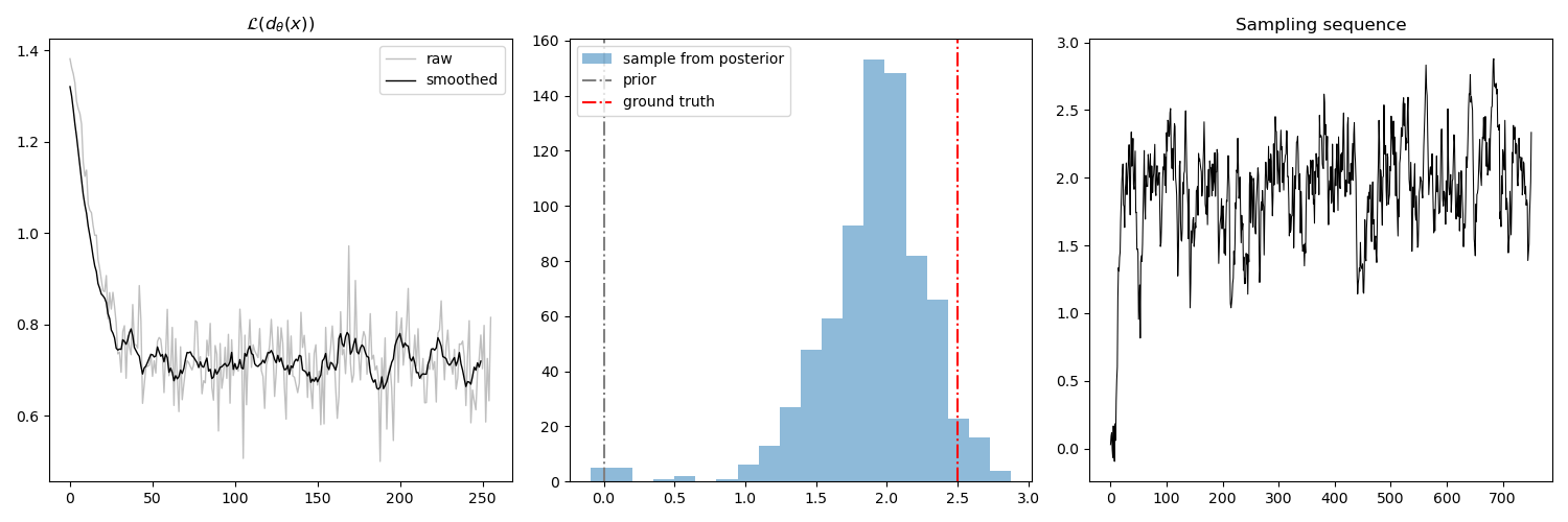
We want to draw samples from the posterior distribution \(p(\theta | \mathbf{x})\), where \(x \sim \mathcal{N}(2.5, 1)\).
Implementation
  1
  2
  3
  4
  5
  6
  7
  8
  9
 10
 11
 12
 13
 14
 15
 16
 17
 18
 19
 20
 21
 22
 23
 24
 25
 26
 27
 28
 29
 30
 31
 32
 33
 34
 35
 36
 37
 38
 39
 40
 41
 42
 43
 44
 45
 46
 47
 48
 49
 50
 51
 52
 53
 54
 55
 56
 57
 58
 59
 60
 61
 62
 63
 64
 65
 66
 67
 68
 69
 70
 71
 72
 73
 74
 75
 76
 77
 78
 79
 80
 81
 82
 83
 84
 85
 86
 87
 88
 89
 90
 91
 92
 93
 94
 95
 96
 97
 98
 99
100
101
102
103
104
105
106
107
108
109
110
111
112
113
114
115
116
117
118
119
120
121
122
123
124
125
126
127
128
129
130
131
132
133
134
135
136
137
138
139
140
141
142
143
144
145
146
147
148
149
150
151
152
153
154
155
156
157
158
159
160
161
162
163
164
165
166
167
168
169
170
171
172
173
174
175
176
177
178
179
180
181
182
183
184
185
186
187
188
189
190
191
192
193
194
195
196
197
198
199
200
201
202
203
204
205
206
import click
import numpy as np
import torch
from matplotlib import pyplot as plt
from torch import nn
from torch.nn import functional as F
from typing import NamedTuple

np.random.seed(1)
torch.manual_seed(1)

def stochastic(func):
    def __wrapper__(*args, **kwargs):
        np.random.seed()
        rs = func(*args, **kwargs)
        np.random.seed(1)
        return rs

    return __wrapper__


class Layer(NamedTuple):
    h: int # hidden dim
    a: str # activation


def Dense(h_i: int, h_j: int, a : str):
    if a == "tanh":
        act = nn.Tanh()
    elif a == "sigmoid":
        act = nn.Sigmoid()
    elif a == "relu":
        act = nn.ReLU()
    else:
        raise NotImplementedError(a)

    return nn.Sequential(
            nn.Linear(h_i, h_j),
            act)


def build_mlp(input_dim: int, seq: list[Layer]) -> nn.Module:
    h0, a0 = seq[0]
    _seq = [Dense(input_dim, h0, a0)]

    for j in range(1, len(seq)):
        h_j, a_j = seq[j]
        h_i, _ = seq[j - 1]
        _seq.append(Dense(h_i, h_j, a_j))

    return nn.Sequential(*_seq)


def train_step(
        Xpos: torch.Tensor,
        Xneg: torch.Tensor,
        d: nn.Module,
        opt: torch.optim.Optimizer) -> torch.Tensor:
    """
    Args:
    - Xpos: (x, theta)
    - Xneg: (x, theta')
    - d: classifier

    Where theta/theta' ~ p, x ~ p(x | theta)
    """
    for i in range(32):
        opt.zero_grad()

        zpos = d(Xpos)
        zneg = d(Xneg)

        loss = F.binary_cross_entropy(zpos, torch.ones_like(zpos))\
                + F.binary_cross_entropy(zneg, torch.zeros_like(zneg))

        loss.backward()
        opt.step()

    return loss.item()


def train_d(
        p: callable,
        sim: callable,
        d: nn.Module,
        m: int,
        e: int,
        lr: float):
    """
    Args:
    - p : prior
    - sim: simulator (implicit p(x | theta)
    - d: parameterized classifier
    - m: batch_size
    - e: max epochs
    - lr: learning rate
    """

    opt = torch.optim.Adam(d.parameters(), lr=lr)
    sch = torch.optim.lr_scheduler.ReduceLROnPlateau(opt)

    losses = []

    for b in range(e):
        theta = p(m)
        theta_prime = p(m)
        x = sim(theta)

        # expand dims everything
        theta = np.expand_dims(theta, -1)
        theta_prime = np.expand_dims(theta_prime, -1)
        x = np.expand_dims(x, -1)

        # construct training sample
        Xpos = np.concatenate([x, theta], -1)
        Xneg = np.concatenate([x, theta_prime], -1)
        Xpos, Xneg = torch.tensor(Xpos, dtype=torch.float),\
                torch.tensor(Xneg, dtype=torch.float)

        loss = train_step(Xpos, Xneg, d, opt)
        losses.append(loss)

        if b%50 == 49:
            sch.step(loss)

    return d, losses


@stochastic
def mcmc(lp: callable, obs: np.ndarray, d: nn.Module, n_samples: int, step_size: float):
    """
    Amortized MCMC likelihood free
    """
    # proposal distribution:
    q = lambda theta: np.random.normal(theta, step_size)

    # initialize theta
    theta = 0.

    samples = []
    obs = np.expand_dims(obs, -1)

    for i in range(n_samples):
        theta_prime = q(theta)

        mu_theta = np.ones_like(obs) * theta
        mu_theta_prime = np.ones_like(obs) * theta_prime

        # construct input vector
        X = np.concatenate([obs, mu_theta], -1)
        Xp = np.concatenate([obs, mu_theta_prime], -1)

        X, Xp= torch.tensor(X, dtype=torch.float),\
                torch.tensor(Xp, dtype=torch.float)

        # Compute the decision function
        d_theta = d(X).detach().mean().numpy()
        d_theta_prime = d(Xp).detach().mean().numpy()

        r_theta = d_theta / (1 - d_theta)
        r_theta_prime = d_theta_prime / (1- d_theta_prime)

        H = r_theta_prime / r_theta
        H = lp(theta_prime) / lp(theta) * H
        H = 1 if H > 1 else H
        u = np.random.uniform()

        if u < H:
            # accept theta_prime
            samples.append(theta_prime)
            theta = theta_prime

    return samples

def main(
        batch_size: int,
        max_iter: int,
        lr: float,
        n_obs: int,
        n_samples: int,
        step_size: float):

    # PROBLEM SETUP
    # --------------------------------------------------
    # prior theta
    p = lambda m: np.random.normal(0, 1, size=m)
    lp = lambda x: np.exp(-0.5 * x**2)#likelihood function

    # simulator: unknown
    sim = lambda mu: np.random.normal(mu, np.ones_like(mu) * .25)

    # parmeterized classifier
    d = build_mlp(
            2, [Layer(4, 'relu'), Layer(2, 'relu'), Layer(1, 'sigmoid')])

    # TRAINING the classifier
    # --------------------------------------------------
    d, losses = train_d(p, sim, d, m=batch_size, e=max_iter, lr=lr)

    # inference
    # --------------------------------------------------
    MU = 2.5 #unknown
    obs = sim(np.ones(n_obs) * MU)

    # Posterior sample: sample p(theta | obs)
    samples = mcmc(lp, obs, d, n_samples, step_size)
Result

